A short project to explore the use of random walk algorithms with the igraph package and make an awesome animation! Random walk algorithms are used to estimate how information spreads across a given graph. An example can be the spread of persons within the walking routes in a theme park. Another applications include the PageRank algorithm, famously invented by Google founder Larry Page to measure the importance of websites.
Here we will try to make a person walk through a graph that for example can be the walking paths in a park. First we will make the graph that represents the park.
library(tidyverse)
library(igraph)
library(gganimate)
library(ggimage)

## make the igraph object
g <- make_graph(~ 1-2, 1-3, 1-4, 4-5, 6-3, 7-6, 5-7, 4-3)

plot(g)
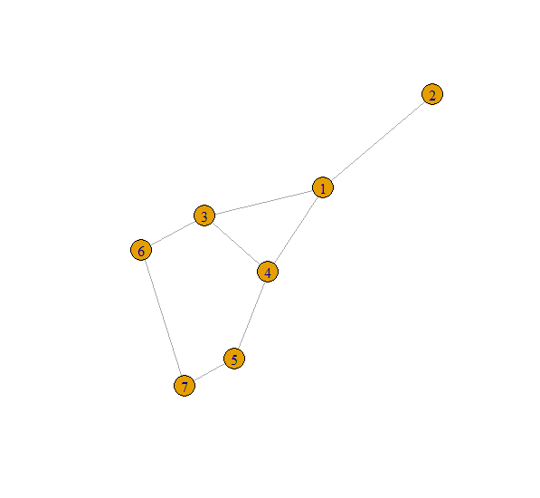 Here we see a simple graph that is our park. We made it by defining all the edges manually. Now let’s walk!
set.seed(20190914)
w <- random_walk(g, start = 2, steps = 15)

w
+ 15/7 vertices, named, from 5bf3145:
[1] 2 1 3 6 3 4 5 7 6 3 1 4 1 2 1
Our walk started at node 2 and then we walked ‘15 steps’ through our park. Can you smell the green, freshly cut grass? Can you hear all the birds sing their hearts out? How lovely!
The random walk algorithm is normally used to simulate thousands or millions of walking paths to better understand the use of space. Although these number sequences require a lot of imagination to understand what is happening. To better explain it to others, we can animate this walk with the ggplot and gganimate packages. First we will build a dataframe these packages can work with. We also save the coordinates of all the nodes.
## animating with ggplot
## make a dataframe with the graph
graph_df <- data_frame(x = c(1.5, 1, 1.5, 3, 1.5, 3, 3, 5, 3, 5, 5, 6, 6, 5, 3, 3),
                       y = c(1.5, 2, 1.5, 2, 1.5, 1, 1, 1, 2, 2, 2, 1.5, 1.5, 1, 2, 1),
                       node = c(1, 2, 1, 3, 1, 4, 4, 5, 3, 6, 6, 7, 7, 5, 3, 4),
                       gr = rep(c(1:8), each = 2))

## saving coordinates of all the nodes
unique_nodes <- graph_df %>%
  distinct(node, .keep_all = TRUE)
Then we take the random walk sequence and join the different coordinates of these nodes to this walking route
## make a dataframe with the random walk order and cordinates of the knots in the graph
rw_order_df <- data.frame(walk = as.vector(w)) %>%
  left_join(unique_nodes, by = c("walk" = "node")) %>%
  mutate(time = row_number())
Now we have the information to plot the full graph and we have the information to animate our walk on top of it. These are essentially the two layers of this plot. With gganimate it is now easy to animate our walk.
a <- ggplot(data = rw_order_df) +
  geom_line(data = graph_df, aes(x, y, group = gr), colour = "lightgrey", size = 2) +
  geom_point(data = graph_df, aes(x, y, group = gr), colour = "orange2", size = 8) +
  ylim(0.95, 2.05) +
  theme_void() +
  ## here we load an emoji to represent us as we walk through the park.
  geom_emoji(data = rw_order_df, aes(x = x, y= y), image = "1f6b6", size = 0.16) +
  ## animation
  transition_states(time, transition_length = 1, state_length = 0.5) +
  ease_aes("sine-in-out")

animate(a, nframes = 300)
anim_save("rw_anim.gif")
With this kind of animation I can easily explain what the random walk algorithm does. Even to people who are not technical at all. Now it is easy to understand what is happening and it is fun to watch. This was certainly a hit with my colleagues!